Application of the YOLO computer vision algorithm

The name YOLO algorithm (You Only Look Once) suggests that it is an algorithm from the subgroup of One-Stage computer vision algorithms. It shares the single-level group together with the SSD (Single Shot Detection) Algorithm which is somewhat more precise than the YOLO algorithm, but also slower. The speed and real-time application are the main advantages and characteristics of the YOLO algorithm.

Other algorithms such as the popular Fast-RCNN and Faster-RCNN belong to the group of Two-Stage algorithms, where the detection of possible object regions takes place at the first level, while the classification takes place at the second level. The need to perform multiple iterations in the same image is what significantly slows down these algorithms, although it results in overall greater result confidence.

How the YOLO algorithm works

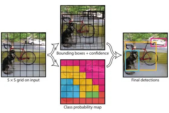
The basis of the YOLO algorithm is that all predictions in a single image take place at once using a fully connected layer. The prediction process can be described with three key steps:

• equal division of the image into N cells, each of which has the same SxS dimension
• prediction of bounding-box coordinates  within each cell for each object, its classification and the probability that the object is located in the cell
• NMS (Non Maximal Suppression) for filtering bounding-boxes in order to leave only one for each object with the highest confidence score of the object class

The key difference between the SSD and the YOLO algorithm is the way the bounding-boxes are regressed. In the mentioned third step of the YOLO algorithm (NMS), the regression of the bounding-boxes takes place by checking for the overlapping bounding-boxes and whether the object classes in them are the same or different. The intersection over union (IoU) principle determines the percentage of bounding-boxes that overlap for the same object class. For overlap above 50%, bounding-boxes which are redundant are eliminated. The centroid of the bounding-box with the average score is selected as the location of the object.

Development of the YOLO algorithm

The basic version of the YOLO algorithm from 2015 had a problem with the detection of smaller grouped objects as well as with the localization accuracy. Next year, the YOLOv2 algorithm would be released, introducing the application of anchor-box regions. While the basic algorithm used a fixed SxS grid where each cell predicted only one object class, the introduction of anchor-boxes enabled the prediction of multiple bounding-boxes for each cell in the SxS grid. This solved the problem of small objects of different classes located inside one cell.

The next step in development was the YOLO9000 algorithm, which aimed to expand the possible classes for detection, that is, from 80 classes of the COCO dataset to 22000 of the ImageNet dataset. As some classes from the COCO dataset hierarchically overlapped with those from ImageNet, the result was somewhere over 9000 possible classes for detection, with the cost of lowering the average precision.

For novelty, YOLOv3 introduces the Darknet-53 as the basis of the network architecture, a more complex model than the previously used DarkNet-19. Also, each cell predicts three bounding-boxes, each of them making an additional prediction at three different scales, leading to a total of nine anchor-boxes per cell.

Further development of YOLO algorithms continues in the form of open-source projects, with the latest version being YOLOv7 in 2022.

Application and comparison of YOLOv3 and YOLOv5 algorithms on store shelves

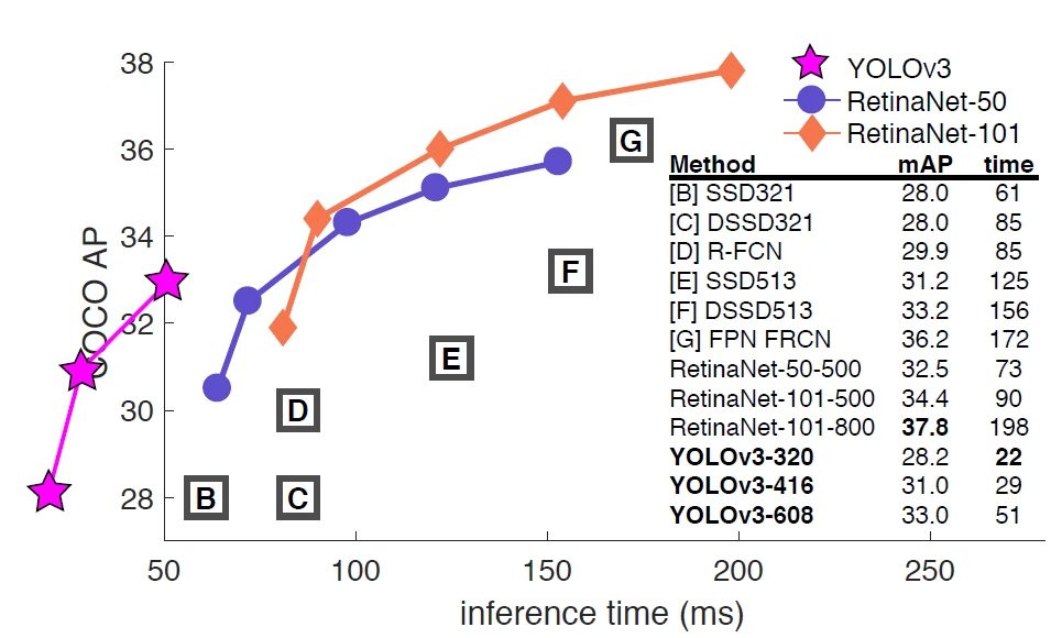
YOLOv3 was released in 2018 and given that it has a well-established base,   it was easy to prepare our database and train the model to recognize store shelves. YOLOv3 has a significantly faster inference time compared to other popular models, but it does not fall far behind even with the average precision.

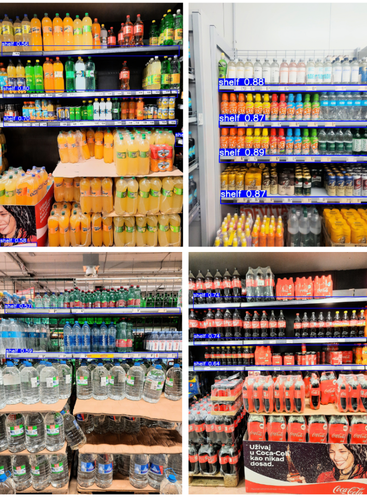
The results shown in Figure 3 were obtained by inference of the trained model on several test photos.

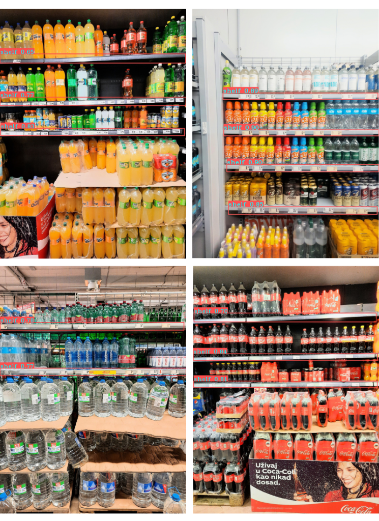
Although YOLOv3 gave extremely satisfactory results on a set of 250 test images, with a very low amount of false positives, we also tried YOLOv5. The main advantage of the YOLOv5 version compared to the YOLOv3 is the speed of training and inference, while the average precision should be more or less the same. After training, the results shown in Figure 4 were obtained.

Conclusion

Based on the papers read that describe and compare the performance of the YOLO algorithms in detail, we came to a choice between two proven algorithms with extensive knowledge bases, namely YOLOv3 and YOLOv5. Although our focus was more on the reliability and precision of the results that the inference execution time, which is the main advantage of all YOLO algorithms, both algorithms proved to be a good choice. The total inference time is slightly shorter with the YOLOv5 model, but it turned out that in the case of shelf recognition it still tends to give a few false positives, while YOLOv3 with slightly lower confidence scores still gave more accurate results.

As with all other computer vision algorithms, due to various unpredictable factors in real-world applications (lighting conditions, human factor), there is not a unique model for every problem, including the problem of store shelf detection. Looking at problems in a wider context, we have to decide what will ultimately result in user satisfaction, because the computer vision algorithm is only one part of the grand scheme, which is our application.

References: